About the CoMSES Model Library more info
Our mission is to help computational modelers at all levels engage in the establishment and adoption of community standards and good practices for developing and sharing computational models. Model authors can freely publish their model source code in the Computational Model Library alongside narrative documentation, open science metadata, and other emerging open science norms that facilitate software citation, reproducibility, interoperability, and reuse. Model authors can also request peer review of their computational models to receive a DOI.
All users of models published in the library must cite model authors when they use and benefit from their code.
Please check out our model publishing tutorial and contact us if you have any questions or concerns about publishing your model(s) in the Computational Model Library.
We also maintain a curated database of over 7500 publications of agent-based and individual based models with additional detailed metadata on availability of code and bibliometric information on the landscape of ABM/IBM publications that we welcome you to explore.
Displaying 10 of 108 results random clear search
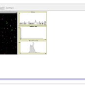
Peer reviewed The Effect of Spatial Clustering on Stone Raw Material Procurement
Simen Oestmo Marco Janssen Curtis W Marean | Published Friday, April 21, 2017This model allows for the investigation of the effect spatial clustering of raw material sources has on the outcome of the neutral model of stone raw material procurement by Brantingham (2003).
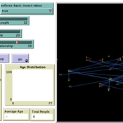
Peer reviewed Monogamous Reproduction in Small Populations and the Enforcement of the Incest Taboo
Ian Stuart | Published Wednesday, January 18, 2023This program was developed to simulate monogamous reproduction in small populations (and the enforcement of the incest taboo).
Every tick is a year. Adults can look for a mate and enter a relationship. Adult females in a Relationship (under the age of 52) have a chance to become pregnant. Everyone becomes not alive at 77 (at which point people are instead displayed as flowers).
User can select a starting-population. The starting population will be adults between the ages of 18 and 42.
…
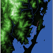
Shellmound Trade
Henrique de Sena Kozlowski | Published Saturday, June 15, 2024This model simulates different trade dynamics in shellmound (sambaqui) builder communities in coastal Southern Brazil. It features two simulation scenarios, one in which every site is the same and another one testing different rates of cooperation. The purpose of the model is to analyze the networks created by the trade dynamics and explore the different ways in which sambaqui communities were articulated in the past.
How it Works?
There are a few rules operating in this model. In either mode of simulation, each tick the agents will produce an amount of resources based on the suitability of the patches inside their occupation-radius, after that the procedures depend on the trade dynamic selected. For BRN? the agents will then repay their owed resources, update their reputation value and then trade again if they need to. For GRN? the agents will just trade with a connected agent if they need to. After that the agents will then consume a random amount of resources that they own and based on that they will grow (split) into a new site or be removed from the simulation. The simulation runs for 1000 ticks. Each patch correspond to a 300x300m square of land in the southern coast of Santa Catarina State in Brazil. Each agent represents a shellmound (sambaqui) builder community. The data for the world were made from a SRTM raster image (1 arc-second) in ArcMap. The sites can be exported into a shapefile (.shp) vector to display in ArcMap. It uses a UTM Sirgas 2000 22S projection system.
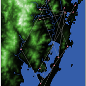
Shellmound Mobility
Henrique de Sena Kozlowski | Published Saturday, June 15, 2024Least Cost Path (LCP) analysis is a recurrent theme in spatial archaeology. Based on a cost of movement image, the user can interpret how difficult it is to travel around in a landscape. This kind of analysis frequently uses GIS tools to assess different landscapes. This model incorporates some aspects of the LCP analysis based on GIS with the capabilities of agent-based modeling, such as the possibility to simulate random behavior when moving. In this model the agent will travel around the coastal landscape of Southern Brazil, assessing its path based on the different cost of travel through the patches. The agents represent shellmound builders (sambaquieiros), who will travel mainly through the use of canoes around the lagoons.
How it works?
When the simulation starts the hiker agent moves around the world, a representation of the lagoon landscape of the Santa Catarina state in Southern Brazil. The agent movement is based on the travel cost of each patch. This travel cost is taken from a cost surface raster created in ArcMap to represent the different cost of movement around the landscape. Each tick the agent will have a chance to select the best possible patch to move in its Field of View (FOV) that will take it towards its target destination. If it doesn’t select the best possible patch, it will randomly choose one of the patches to move in its FOV. The simulation stops when the hiker agent reaches the target destination. The elevation raster file and the cost surface map are based on a 1 Arc-second (30m) resolution SRTM image, scaled down 5 times. Each patch represents a square of 150m, with an area of 0,0225km². The dataset uses a UTM Sirgas 2000 22S projection system. There are four different cost functions available to use. They change the cost surface used by the hikers to navigate around the world.
Agent-based tax evasion model for investigating impacts of public disclosure
Hiroyuki Sano | Published Thursday, March 14, 2024The model explores the impact of public disclosure on tax compliance among diverse agents, including individual taxpayers and a tax authority. It incorporates heterogeneous preferences and income endowments among taxpayers, captured through a utility function that considers psychic costs subtracted from expected pecuniary utility. These costs include moral, reciprocity, and stigma costs associated with norm violations, leading to variations in taxpayers’ risk attitudes and related parameters. The tax authority’s attributes, such as the frequency of random audits, penalty rate, and the choice between partial or full disclosure, remain fixed throughout the simulation. Income endowments and preference parameters are randomly assigned to taxpayers at the outset.
Taxpayers maximize their expected utility by reporting income, taking into account tax, penalty, and audit rates. They make annual decisions based on their own and their peers’ behaviors from the previous year. Taxpayers indirectly interact at the societal level through public disclosure conducted by the tax authority, exchanging tax information among peers. Each period in the simulation collects data on total reported income, average compliance rates per income group, distribution of compliance rates, counts of compliers, full evaders, partial evaders, and the numbers of taxpayers experiencing guilt and anger. The model evaluates whether public disclosure positively or negatively impacts compliance rates and quantifies this impact based on aggregated individual reporting behaviors.
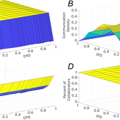
Role of Diversity in Team Performance: the Case of Missing Expertise, an Agent Based Simulations
Tamás Kiss | Published Friday, December 29, 2023This ABM simulates problem solving agents as they work on a set of tasks. Each agent has a trait vector describing their skills. Two agents might form a collaboration if their traits are similar enough. Tasks are defined by a component vector. Agents work on tasks by decreasing tasks’ component vectors towards zero.
The simulation generates agents with given intrapersonal functional diversity (IFD), and dominant function diversity (DFD), and a set of random tasks and evaluates how agents’ traits influence their level of communication and the performance of a team of agents.
Modeling results highlight the importance of the distributions of agents’ properties forming a team, and suggests that for a thorough description of management teams, not only diversity measures based on individual agents, but an aggregate measure is also required.
…
Informal risk-sharing cooperatives : ORP and Learning
Victorien Barbet Renaud Bourlès Juliette Rouchier | Published Monday, February 13, 2017 | Last modified Tuesday, May 16, 2023The model studies the dynamics of risk-sharing cooperatives among heterogeneous farmers. Based on their knowledge on their risk exposure and the performance of the cooperative farmers choose whether or not to remain in the risk-sharing agreement.
Correlated random walk (Javascript)
Thibault Fronville Viktoriia Radchuk Uta Berger | Published Tuesday, May 09, 2023The first simple movement models used unbiased and uncorrelated random walks (RW). In such models of movement, the direction of the movement is totally independent of the previous movement direction. In other words, at each time step the direction, in which an individual is moving is completely random. This process is referred to as a Brownian motion.
On the other hand, in correlated random walks (CRW) the choice of the movement directions depends on the direction of the previous movement. At each time step, the movement direction has a tendency to point in the same direction as the previous one. This movement model fits well observational movement data for many animal species.
The presented agent based model simulated the movement of the agents as a correlated random walk (CRW). The turning angle at each time step follows the Von Mises distribution with a ϰ of 10. The closer ϰ gets to zero, the closer the Von Mises distribution becomes uniform. The larger ϰ gets, the more the Von Mises distribution approaches a normal distribution concentrated around the mean (0°).
In this script the turning angles (following the Von Mises distribution) are generated based on the the instructions from N. I. Fisher 2011.
This model is implemented in Javascript and can be used as a building block for more complex agent based models that would rely on describing the movement of individuals with CRW.
Biodiversity and Adoption of Small-scale Agroforestry in Rwanda (BASAR)
Beatrice Nöldeke Etti Winter Elisée Bahati Ntawuhiganayo | Published Friday, July 15, 2022The BASAR model aims to investigate different approaches to describe small-scale farmers’ decision-making in the context of diversified agroforestry adoption in rural Rwanda. Thereby, it compares random behaviour with perfect rationality (non-discounted and discounted utility maximization), bounded rationality (satisficing and fast and frugal decision tree heuristics), Theory of Planned Behaviour, and a probabilistic regression-based approach. It is aimed at policy-makers, extension agents, and cooperatives to better understand how rural farmers decide about implementing innovative agricultural practices such as agroforestry and at modelers to support them in selecting an approach to represent human decision-making in ABMs of Social-Ecological Systems. The overall objective is to identify a suitable approach to describe human decision-making and therefore improve forecasts of adoption rates and support the development and implementation of interventions that aim to raise low adoption rates.
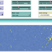
ABM for Underwater optical wireless communication in a water tank
Mohamed ABID | Published Sunday, May 29, 2022This model simulates the propagation of photons in a water tank. A source of light emits an impulse of photons with equal energy represented by yellow dots. These photons are then scattered by water particles before possibly reaching the photo-detector represented by a gray line. Different types of water are considered. For each one of them we calculate the total received energy.
The water tank is represented by a blue rectangle with fixed dimensions. It’s exposed to the air interface and has totally absorbent barriers. Four types of water are supported. Each one is characterized by its absorption and scattering coefficients.
At the source, the photons are generated uniformly with a random direction within the beamwidth. Each photon travels a random distance drawn from a distribution depending on the water characteristics before encountering a water particle.
Based on the updated position of the photon, three situations may occur:
-The photon hits the barrier of the tank on its trajectory. In this case it’s considered as lost since the barriers are assumed totally absorbent.
…
Displaying 10 of 108 results random clear search